Examples

Digital hologram of a single cell

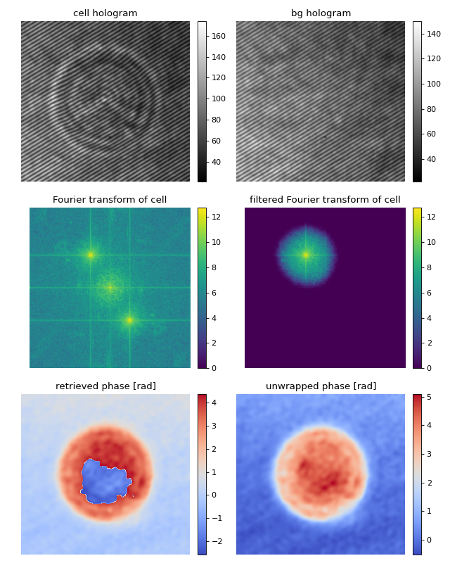
This example illustrates how qpretrieve can be used to analyze digital holograms. The hologram of a single myeloid leukemia cell (HL60) was recorded using off-axis digital holographic microscopy (DHM). Because the phase-retrieval method used in DHM is based on the discrete Fourier transform, there always is a residual background phase tilt which must be removed for further image analysis. The setup used for recording these data is described in reference [SSM+15].

Note that the fringe pattern in this particular example is over-sampled in real space, which is why the sidebands are not properly separated in Fourier space. Thus, the filter in Fourier space is very small which results in a very low effective resolution in the reconstructed phase.

hologram_cell.py

import matplotlib.pylab as plt
import numpy as np
import qpretrieve
from skimage.restoration import unwrap_phase

# load the experimental data
edata = np.load("./data/hologram_cell.npz")

holo = qpretrieve.OffAxisHologram(data=edata["data"])
holo.run_pipeline(
    # For this hologram, the "smooth disk"
    # filter yields the best trade-off
    # between interference from the central
    # band and image resolution.
    filter_name="smooth disk",
    # Set the filter size to half the distance
    # between the central band and the sideband.
    filter_size=1/2)
bg = qpretrieve.OffAxisHologram(data=edata["bg_data"])
bg.process_like(holo)

phase = holo.phase - bg.phase

# plot the intermediate steps of the analysis pipeline
fig = plt.figure(figsize=(8, 10))

ax1 = plt.subplot(321, title="cell hologram")
map1 = ax1.imshow(edata["data"], interpolation="bicubic", cmap="gray")
plt.colorbar(map1, ax=ax1, fraction=.046, pad=0.04)

ax2 = plt.subplot(322, title="bg hologram")
map2 = ax2.imshow(edata["bg_data"], interpolation="bicubic", cmap="gray")
plt.colorbar(map2, ax=ax2, fraction=.046, pad=0.04)

ax3 = plt.subplot(323, title="Fourier transform of cell")
map3 = ax3.imshow(np.log(1 + np.abs(holo.fft_origin)), cmap="viridis")
plt.colorbar(map3, ax=ax3, fraction=.046, pad=0.04)

ax4 = plt.subplot(324, title="filtered Fourier transform of cell")
map4 = ax4.imshow(np.log(1 + np.abs(holo.fft_filtered)), cmap="viridis")
plt.colorbar(map4, ax=ax4, fraction=.046, pad=0.04)

ax5 = plt.subplot(325, title="retrieved phase [rad]")
map5 = ax5.imshow(phase, cmap="coolwarm")
plt.colorbar(map5, ax=ax5, fraction=.046, pad=0.04)

ax6 = plt.subplot(326, title="unwrapped phase [rad]")
map6 = ax6.imshow(unwrap_phase(phase), cmap="coolwarm")
plt.colorbar(map6, ax=ax6, fraction=.046, pad=0.04)

# disable axes
[ax.axis("off") for ax in [ax1, ax2, ax3, ax4, ax5, ax6]]

plt.tight_layout()
plt.show()

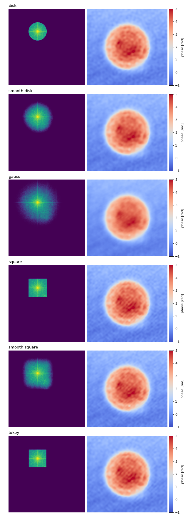
Filter visualization

This example visualizes the different Fourier filtering masks available in qpretrieve.

filter_visualization.py

import matplotlib.pylab as plt
import numpy as np
import qpretrieve
from skimage.restoration import unwrap_phase

# load the experimental data
edata = np.load("./data/hologram_cell.npz")

prange = (-1, 5)
frange = (0, 12)

results = {}

for fn in qpretrieve.filter.available_filters:
    holo = qpretrieve.OffAxisHologram(data=edata["data"])
    holo.run_pipeline(
        filter_name=fn,
        # Set the filter size to half the distance
        # between the central band and the sideband.
        filter_size=1/2)
    bg = qpretrieve.OffAxisHologram(data=edata["bg_data"])
    bg.process_like(holo)
    phase = unwrap_phase(holo.phase - bg.phase)
    mask = np.log(1 + np.abs(holo.fft_filtered))
    results[fn] = mask, phase

num_filters = len(results)

# plot the properties of `qpi`
fig = plt.figure(figsize=(8, 22))

for row, name in enumerate(results):
    ax1 = plt.subplot(num_filters, 2, 2*row+1)
    ax1.set_title(name, loc="left")
    ax1.imshow(results[name][0], vmin=frange[0], vmax=frange[1])

    ax2 = plt.subplot(num_filters, 2, 2*row+2)
    map2 = ax2.imshow(results[name][1], cmap="coolwarm",
                      vmin=prange[0], vmax=prange[1])
    plt.colorbar(map2, ax=ax2, fraction=.046, pad=0.02, label="phase [rad]")

    ax1.axis("off")
    ax2.axis("off")

plt.tight_layout()
plt.show()

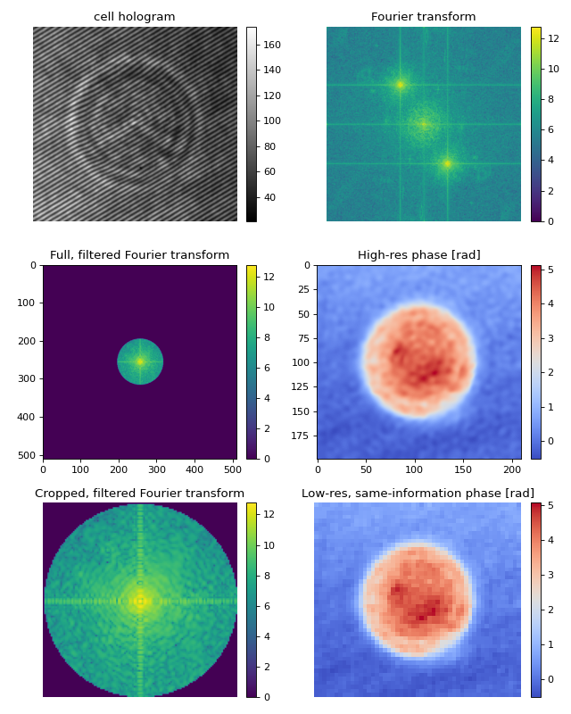
Adequate resolution-scaling via cropping in Fourier space

Applying filters in Fourier space usually means setting a larger fraction of the data in Fourier space to zero. This can considerably slow down your analysis, since the inverse Fouier transform is taking into account a lot of unused frequencies.

By cropping the Fourier domain, the inverse Fourier transform will be faster. The result is an image with fewer pixels (lower resolution), that contains the same information as the unscaled (not cropped in Fourier space) image. There are possibly two disadvantages of performing this cropping operation:

1. The resolution of the output image (pixel size) is not the same as that of the input (interference) image. Thus, you will have to adapt your colocalization scheme.

2. If you are using a filter with a non-binary mask (e.g. gauss), then you will lose (little) information when cropping in Fourier space.

What happens when you set filter_name=”smooth disk”? Cropping with scale_to_filter=True is too narrow, because now there are higher frequencies contributing to the final image. To include them, you can set scale_to_filter to a float, e.g. scale_to_filter=1.2.

fourier_scale.py

import matplotlib.pylab as plt
import numpy as np
import qpretrieve
from skimage.restoration import unwrap_phase

# load the experimental data
edata = np.load("./data/hologram_cell.npz")

results = []

holo = qpretrieve.OffAxisHologram(data=edata["data"])
bg = qpretrieve.OffAxisHologram(data=edata["bg_data"])
ft_orig = np.log(1 + np.abs(holo.fft_origin), dtype=float)

holo.run_pipeline(filter_name="disk", filter_size=1/2,
                  scale_to_filter=False)
bg.process_like(holo)
phase_highres = unwrap_phase(holo.phase - bg.phase)
ft_highres = np.log(1 + np.abs(holo.fft.fft_used), dtype=float)

holo.run_pipeline(filter_name="disk", filter_size=1/2,
                  scale_to_filter=True)
bg.process_like(holo)
phase_scalerad = unwrap_phase(holo.phase - bg.phase)
ft_scalerad = np.log(1 + np.abs(holo.fft.fft_used), dtype=float)

# plot the intermediate steps of the analysis pipeline
fig = plt.figure(figsize=(8, 10))

ax1 = plt.subplot(321, title="cell hologram")
map1 = ax1.imshow(edata["data"], interpolation="bicubic", cmap="gray")
plt.colorbar(map1, ax=ax1, fraction=.046, pad=0.04)

ax2 = plt.subplot(322, title="Fourier transform")
map2 = ax2.imshow(ft_orig, cmap="viridis")
plt.colorbar(map2, ax=ax2, fraction=.046, pad=0.04)

ax3 = plt.subplot(323, title="Full, filtered Fourier transform")
map3 = ax3.imshow(ft_highres, cmap="viridis")
plt.colorbar(map3, ax=ax3, fraction=.046, pad=0.04)

ax4 = plt.subplot(324, title="High-res phase [rad]")
map4 = ax4.imshow(phase_highres, cmap="coolwarm")
plt.colorbar(map4, ax=ax4, fraction=.046, pad=0.04)

ax5 = plt.subplot(325, title="Cropped, filtered Fourier transform")
map5 = ax5.imshow(ft_scalerad, cmap="viridis")
plt.colorbar(map5, ax=ax5, fraction=.046, pad=0.04)

ax6 = plt.subplot(326, title="Low-res, same-information phase [rad]")
map6 = ax6.imshow(phase_scalerad, cmap="coolwarm")
plt.colorbar(map6, ax=ax6, fraction=.046, pad=0.04)

# disable axes
[ax.axis("off") for ax in [ax1, ax2, ax5, ax6]]

plt.tight_layout()
plt.show()

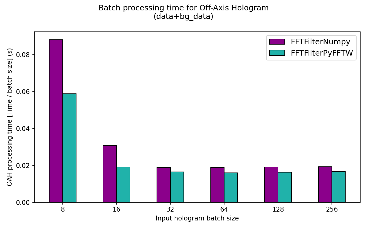
Fourier Transform speed benchmarks for OAH

This example visualizes the speed for different batch sizes for the available FFT Filters. The y-axis shows the average speed of a pipeline run for the Off-Axis Hologram class OffAxisHologram, including background data processing. Therefore, four FFTs are run per pipeline.

• Optimum batch size is between 64 and 256 for 256x256pix imgs (incl padding), but will be limited by your computer’s RAM.

• Here, batch size is the size of the 3D stack in z.

• Note that each pipeline runs 4 FFTs. For example, batch 8 runs 8*4=32 FFTs.

fft_batch_speeds.py

import time
import matplotlib.pylab as plt
import numpy as np
import qpretrieve
from qpretrieve.data_array_layout import convert_data_to_3d_array_layout
from qpretrieve.fourier import FFTFilterNumpy, FFTFilterPyFFTW

# load the experimental data
edata = np.load("./data/hologram_cell.npz")

n_transforms_list = [8, 16, 32, 64, 128, 256]
subtract_mean = True
padding = True
# we take the PyFFTW speeds from the second run
fft_interfaces = [FFTFilterNumpy, FFTFilterPyFFTW, FFTFilterPyFFTW]
filter_name = "disk"
filter_size = 1 / 2
speed_norms = {}

# load and prep the data
data_2d = edata["data"].copy()
data_2d_bg = edata["bg_data"].copy()
data_3d_prep, _ = convert_data_to_3d_array_layout(data_2d)
data_3d_bg_prep, _ = convert_data_to_3d_array_layout(data_2d_bg)

for fft_interface in fft_interfaces:
    results = {}
    for n_transforms in n_transforms_list:
        print(f"Running {n_transforms} transforms with "
              f"{fft_interface.__name__}")

        # create batches
        data_3d = np.repeat(data_3d_prep, repeats=n_transforms, axis=0)
        data_3d_bg = np.repeat(data_3d_bg_prep, repeats=n_transforms, axis=0)

        assert data_3d.shape == data_3d_bg.shape == (n_transforms,
                                                     edata["data"].shape[0],
                                                     edata["data"].shape[1])

        t0 = time.time()
        holo = qpretrieve.OffAxisHologram(data=data_3d,
                                          fft_interface=fft_interface,
                                          subtract_mean=subtract_mean,
                                          padding=padding)
        holo.run_pipeline(filter_name=filter_name, filter_size=filter_size)
        bg = qpretrieve.OffAxisHologram(data=data_3d_bg)
        bg.process_like(holo)
        t1 = time.time()
        results[n_transforms] = t1 - t0

    speed_norm = [timing / b_size for b_size, timing in results.items()]
    # the initial PyFFTW run (incl wisdom calc is overwritten here)
    speed_norms[fft_interface.__name__] = speed_norm

# setup plot
fig, axes = plt.subplots(1, 1, figsize=(8, 5))
ax1 = axes
width = 0.25  # the width of the bars
multiplier = 0
x_pos = np.arange(len(n_transforms_list))
colors = ["darkmagenta", "lightseagreen"]

for (name, speed), color in zip(speed_norms.items(), colors):
    offset = width * multiplier
    ax1.bar(x_pos + offset, speed, width, label=name,
            color=color, edgecolor='k')
    multiplier += 1

ax1.set_xticks(x_pos + (width / 2), labels=n_transforms_list)
ax1.set_xlabel("Input hologram batch size")
ax1.set_ylabel("OAH processing time [Time / batch size] (s)")
ax1.legend(loc='upper right', fontsize="large")

plt.suptitle("Batch processing time for Off-Axis Hologram\n"
             "(data+bg_data)")
plt.tight_layout()
# plt.show()
plt.savefig("fft_batch_speeds.png", dpi=150)